Having finished the first semester at the university, I’ve gotten to know TikZ, for drawing figures and graphs, when typesetting in LaTeX. One might argue that TikZ isn’t used to draw figures, as it’s a recursive acronym meaning “TikZ ist kein Zeichenprogramm”, translating to “TikZ is not a drawing program”. And sure, TikZ isn’t in any way a WYSIWYG, has a somewhat steep learning curve, and small changes can take a long time to recompile. On the other hand, TikZ is built around LaTeX, meaning it offers superior typegraphy, precise positioning, and extensive macros.

There are many different ways to draw pictures in TikZ, I will try to cover some of them. The PGF/TikZ Manual covers way more content, and has great examples included.

Getting started

We start by including the TikZ package in the preamble, and loading the optional libraries along with it.

\usepackage{tikz}
\usetikzlibrary{library1, library2}

Some libraries include

• arrows.meta
• calc
• intersections
• mindmap
• positioning
• shapes

TikZ can be used both inline, and as an environment.

Inline

\tikz[options]{commands}

Environment

\begin{tikzpicture}[options]
    commands
\end{tikzpicture}

For this introduction, I will focus on the latter.

Drawing using coordinates

We can draw lines in TikZ from coordinates, specifying the position of the pen, and where to move to next.

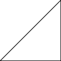
\draw (0,0) -- (2,0) -- (2,2) -- cycle;

Specifying --, means the line is drawn directly, and then the next coordinate is given. cycle returns back the origin of the \draw command.

This produces the following figure:

Coordinates can also be given relative to the last one, and with units specified.

\draw (1cm,5mm) -- (-1cm, 50pt) -- ++(2,0);

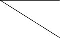
++(2,0) moves the pen 2 units in the x-direction and 0 in the y-direction, relative to the last position. It’s also possible to use the +(2,0) notation, this also moves relative to the last given coordinate, but does not change the end coordinate of the pen. This means that a square would could be drawn like such:

\draw (-2cm, 1in) -- +(1,0) -- +(1,1) -- +(0,1) -- cycle;

Units can be specified using most of the default LaTeX units.

This can also be simplified, using the rectangle keyword.

\draw (-2cm, 1in) rectangle +(1,1);

Here we specify two diagonally opposite corners, to create an identical square to the previous command, with side lengths 1, originating from (-2cm,1in).

Customizing \draw

The line drawn can be customized using various options for the \draw command.

\draw[blue, very thick, dashed] (0,1) circle (45pt);

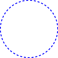
The color is specified from the default colors in LaTeX. If xcolor is loaded, it’s also possible to draw in any of these colors (or any other custom set). The thickness is set to some value in the range of ultra thin, very thin, thin (default), semithick, thick, very thick, ultra thick. Lastly, we tell TikZ to make the line dashed. One could also have opted for the dotted option.

The circle itself is draw using a center, the circle keyword, followed by a radius.

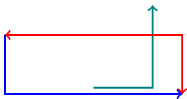
The lines drawn can also be changed to arrows, by specifying either ->, <- or <->, depending on which direction it should point.

We see this along with the -| and |- options for connecting coordinates. This makes the line follow the x- and y-axis, instead of drawing a straight line.

\draw[thick, teal, ->]   (0,3pt) -| (1,1.5);
\draw[thick, red, <->]   (1.5,0) |- +(-3,1); 
\draw[thick, blue, <-]   (1.5,0) -| +(-3,1); % same coordinates as above

Returning to our rectangle, we see that this can once again be drawn in a new way:

\draw (0,0) -| (1,1) -| cycle;

This is again done by using the two diagonally opposite corners

Nodes and edges

Nodes are used to draw text on the canvas, and can be placed using coordinates, or a position relative to another object.

We will start by looking at an example, showing some of the functionality of nodes and edges.

\usetikzlibrary{shapes.geometric}
% needed for diamond and star shape

\begin{tikzpicture}
\node[draw, circle]                (a) at (0,1.5)   {$x$};
\node[draw, diamond, red]          (b) at (1.5,1.5) {B};
\node[draw, star, fill=yellow!30]  (c) at (0,0)     {};
\node                              (d) at (1.5,0)   {Node 4};

\draw[violet] (a) -- (b) -- (d);
\draw[->]     (c) -- (b) edge[bend left] (d)
              (a) edge[out=-30, in=-135, thick] (d);
\end{tikzpicture}

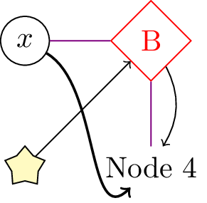
Each node is drawn, using the \node command, with options directly after. Then we assign it a name, and a location using coordinates, exactly the same way as when we were drawing previously. Lastly, we write the “content” of the node. This is optional, but can also take comprehensive arguments, like math equations, and stylings of text (like \texttt, and \textbf).

After having placed the nodes, we begin drawing paths between them. We see that this is almost the same as we did earlier, but this time we only specify the node name, instead of coordinates.

To manipulate these edges, we use the edge keyword instead of --, this allows us to customize the behaviour of the specific edge. In the above example, I’ve shown how to bend the edge slightly (node b to d), and how to specify the angle of exit and entry on each node (node a to d).

Furthermore, we also see that this code requires a library to compile. The shape library, contains a lot of more advanced shapes, for us to use.

Positioning

We can also place nodes and edges at the same time. This is useful for describing some edge with text or other graphics.

\usetikzlibrary{positioning}

\begin{tikzpicture}[
blob/.style={draw,circle},
node distance=1cm,
]

\node [blob]                      (1) at (1,1) {1};
\node [blob, above right=of 1]             (2) {2};
\node [blob, right=of 1]                   (3) {3};
\node [blob, below=of 1]                   (4) {4};
\node [blob, below right=1cm and 2cm of 3] (5) {5};

\draw[red] (3.5cm,1.5cm) -- node [above] {1cm} +(1cm,0);

\draw[yellow!20!blue]
(1) -- node[above, sloped]             {1cm} (2)
(1) -- node[above]                     {1cm} (3)
(1) -- node[right]                     {1cm} (4)
(3) -- node[above, sloped]             {$\sqrt{5}$cm} (5)
(3) |- node[above, sloped, near start] {1cm}
       node[below, near end]           {2cm} (5);
\end{tikzpicture}

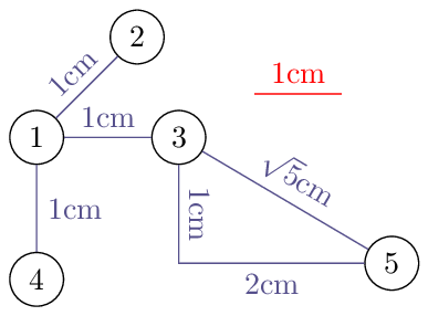
Here we see some options, loaded in the tikzpicture environment. First we create a new style, named blob, using the /.style= syntax, this style holds the properties draw, circle. We also specify the default distance between nodes, this is used when placing nodes relative to one another.

The positioning library enables us to place nodes this way. We see this, when drawing node 2-5. They are all placed relative to a previously placed node. For node 5, we change the distance, from the default, to 1 cm in the y direction, and 2 cm in the x direction. All of the relative placements are done using the below / above / left / right = of <node/coordinate> syntax. To place node b north west of node a, we write above left=of a in the properties of b.

Note: The x, and y offsets are in opposite order, because we must specify below/above, prior to left/right.

Furthermore, we can choose, where on the path, the node should be, this is done with arguments containing start and end.

Anchors

Every node has anchors, which all refer to a certain point on the node. Previously, when we specified right=10pt of <node>, TikZ sets the distance between the new nodes .west anchor, and <node>.east, to 10 pt.

To illustrate this, we look at one of the examples, from the shapes library.

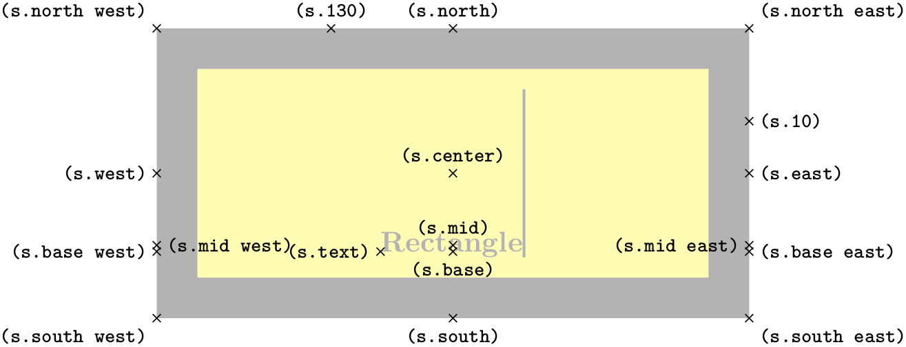
Here we see that the rectangle holds numerous of values, which can all be referenced. The s.10 and s.130, are both angles, in degrees, and point to some anchor along the edge of the node, corresponding to said angle. Any angle can be used for this (even negative ones, or ones greater than 360).

.center is the center of the node, .mid is the middle of the text, .base is the baseline of the text, and .text is the bottom left corner of the textbox.

Creating a flowchart

Combining all of this, we can create a small flowchart

\usetikzlibrary{shapes, positioning}

\begin{tikzpicture}[
  arrow/.style={thick, ->},
  item/.style={draw, minimum height=.75cm, minimum width=3cm, centered},
  startstop/.style={item, fill=black!30, rounded rectangle},
  process/.style={item, fill=red!30, rectangle},
  check/.style={item, fill=green!30, diamond},
  io/.style={item, fill=blue!30, trapezium, 
    trapezium left angle=70, trapezium right angle=110}
]

\node (start)  [startstop]                                     {Start};
\node (input)  [io, below=of start]                            {Input};
\node (valid)  [process, below=of input]              {Validate input};
\node (check)  [check, below right=.5 and 1.5 of valid] {Is input OK?};
\node (proc)   [process, below=3 of valid]             {Process Input};
\node (output) [io, below=of proc]                            {Output};
\node (end)    [startstop, below=of output]                      {End};

\draw[arrow] (start)  -- (input);
\draw[arrow] (input)  -- (valid);
\draw[arrow] (valid)  |- (check);
\draw[arrow] (proc)   -- (output);
\draw[arrow] (output) -- (end);
\draw[arrow] (check)  |- node[very near start, right] {No} (input);
\draw[arrow] (check.south) -- ++(0, -5pt)
    -| node[above, near start] {Yes} (proc.north);
\end{tikzpicture}

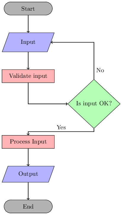
Adding new elements to this is easy, since we have already predefined some symbols to use. Adding the text width=<value> property could be useful, for extensive elements, with lots of text, as this limits the width of the text, before wrapping it.

Summing up

This short introduction only covers a fraction of what TikZ can do. TikZ can also be used to draw graphs, plotting functions (even 3D ones), making mindmaps, visualize just about any type of data, and much, much more. Hopefully this has given you a better understanding of what TikZ can be used for, and of course how it can be used.

The best way to learn it, is to jump right in, and start using it!